Fuhad Abdulla
Using real-world e-commerce data, we’ll build a predictive model that helps understand what drives customer spending.
In this project, we’ll explore:
- How time spent on websites versus mobile apps affects purchasing behavior
- The crucial role of membership duration in customer spending
- Visual analysis of customer engagement patterns
- Building and evaluating a Linear Regression model.
Regression Plot using actual Values
The plot created by sns.lmplot is a regression plot, which is a type of plot used to visualize the relationship between two continuous variables along with a fitted linear regression line.
sns.lmplot(x='Length of Membership',y='Yearly Amount Spent',data=df,scatter_kws={'alpha':0.4})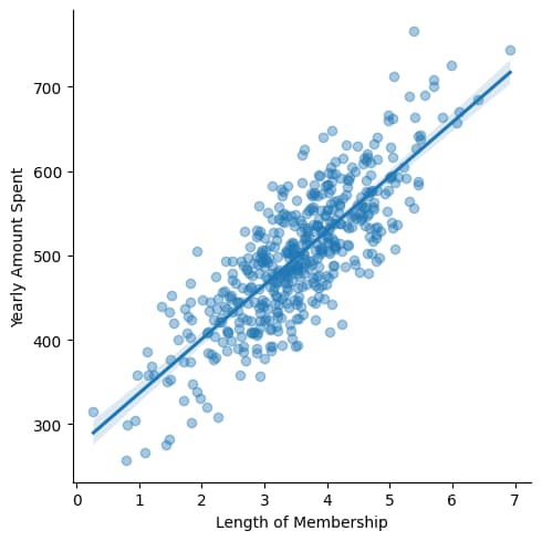
Following the prediction made by our regression model. In this article we will train the machine learning model and then evaluate it for accuracy.
Final Result Linear Regression Prediction Using LM Model
Complete Code and It’s Explanation
Importing Libraries & Data
import pandas as pd
import matplotlib.pyplot as plt
import seaborn as sns

# here we imported
# pandas is used to interact with dataframe, clean the data, find means, read files
# matplotlib and seaborn are used to create visualisation
df=pd.read_csv('ecommerce.csv')

# here we are creating a dataframe df by reading the ecommerce data which is in csv format
df.head()
# it shows first few row, we can also specify how many row to be shows like df.head(10)df.info()
# It shows information about the data frame like non null count data type, column names df.describe()
# It creates statistical summary like count, mean, standard deviation, minimumn value, maximum value Exploratory Data Analysis
#Exploratory Data Analysis
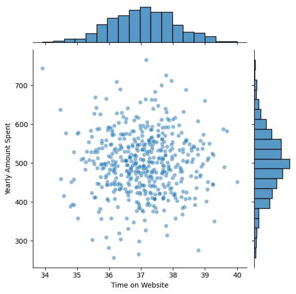
sns.jointplot(x='Time on Website',y="Yearly Amount Spent", data=df,alpha=0.5)
# Using Seaborn to create a plot which is a combination of histogram(distribution plot) and scatter plot between two variable
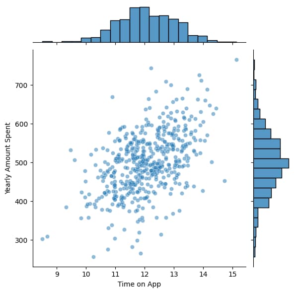
sns.jointplot(x='Time on App',y="Yearly Amount Spent", data=df,alpha=0.5)

# Using Seaborn to create a plot which is a combination of histogram(distribution plot) and scatter plot between two variable
sns.pairplot(df, kind='scatter', plot_kws={'alpha': 0.4})
# show various plots which show relationship between various variable in the dataframe
# if the variable is same on y and x axis it shows the histogram
# helped to see all possible relationship 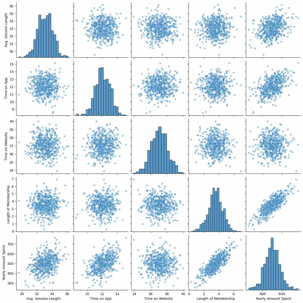
Creating Scatter Plot with Regression Line (Length of Membership & Yearly Amount Spend)
sns.lmplot(x='Length of Membership',y='Yearly Amount Spent',data=df,scatter_kws={'alpha':0.4})

# scatter plot along with regresstion line , 
Splitting Dataset to Training & Testing the Final Prediction.
from sklearn.model_selection import train_test_split

# this is imported to split the dataset to training and testing set
X=df[['Avg. Session Length','Time on App','Time on Website','Length of Membership']]
y=df['Yearly Amount Spent']
# creating variable for our model
# X independent variable
# y dependent variable
# when we train the model we are trying to predict the y Which is yearly amount spend
X_train,X_test,y_train,y_test=train_test_split(X,y,test_size=0.3,random_state=42)

# splitting the data for training and testing
X_train
# show the training datafrom sklearn.linear_model import LinearRegression
# importing the linear regression model from the scikit-learnlm=LinearRegression()
# creating an model instanceTraining the Model with Training Dataset
lm.fit(X_train,y_train)
# Training the LinearRegression model with our data
Checking which variable highest impact on target Value
lm.coef_

# Show the array of coefficient, how much each variable impact the target value
cdf=pd.DataFrame(lm.coef_,X.columns,columns=['Coef'])
print(cdf)
# Coefficient with higher value has more impact so in this case Lenght of Membership has higher impact on the outputTesting the Model with test data
#prediction

predictions=lm.predict(X_test)
predictions

# testing the model with X_test values
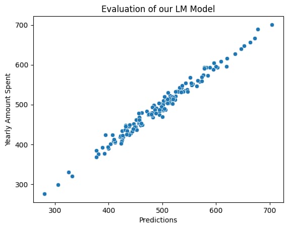
Linear Regression Prediction Using LM Model vs Actual
# we are testing whether the predictions that the trained model give is similar to the actual

#y_test is the actual y

# If it is similar then our model is pretty good for using

sns.scatterplot(x=predictions,y=y_test)
plt.xlabel('Predictions')
plt.title('Evaluation of our LM Model')
The prediction and actual seems to correlating.
Evaluating the Model for Accuracy
from sklearn.metrics import mean_squared_error, mean_absolute_error
import math
# Mean Absolute error check the error in our case it is not bad, mean of yearly amount spend is 500, so error of 8 unit is pretty good
#Average distance between the line and the point of scatter
print('Mean Absolute Error:',mean_absolute_error(y_test,predictions)) # it is like the precictions is off by this much unit
print('Mean Squared Error:',mean_squared_error(y_test,predictions)) # Show larger error
print('Root Mean Squared Error:',math.sqrt(mean_squared_error(y_test,predictions)))
# These help us know whether our model need more improvement or not.residuals=y_test-predictions
# Checking How far off each prediction was
# residuals should be random, if not there is some problems or biasessns.displot(residuals,bins=30,kde=True)
# plot to check the randomness
# A good model should have
# Symmetric distribution
# No unusual pattern
# Bell Shape
# No Multiple peaks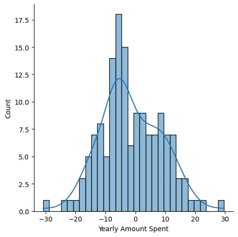
import pylab
import scipy.stats as stats
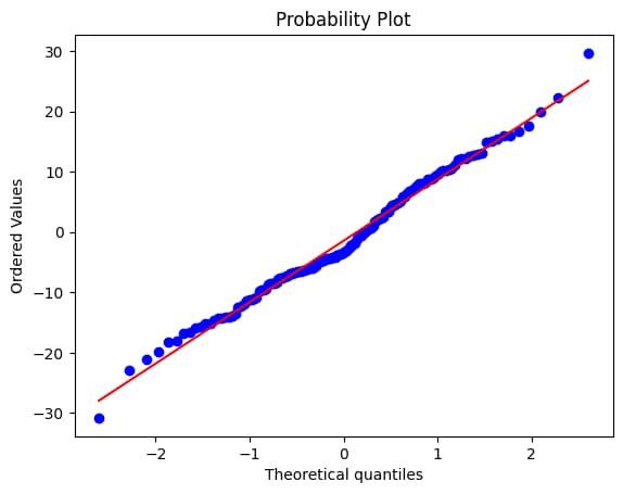
stats.probplot(residuals,dist="norm",plot=pylab)
# checking whether the residual has normal distribution using Q-Q Plot
# if curved line the data is skewed
# Point far from line - Outlier
# Poitn should close to the diagnal line
#
Conclusion
Here we get lm.coef_ (coefficient)
X = customers[[‘Avg. Session Length’, ‘Time on App’, ‘Time on Website’, ‘Length of Membership’]]
Result of lm.coef_
array([25.72425621, 38.59713548, 0.45914788, 61.67473243])
That means Variables which has biggest impact on the Yearly Amount spend is Length of Membership>Time on App>Avg. Session Length>Time on Website
The model in this example has a low prediction error, which means it works well. Using features like Avg. Session Length, Time on App, Time on Website, and Length of Membership, we can reliably predict which variable has the greatest impact on the target which is yearly customer spend.
In this case we find that Length of Membership has the greatest impact on the yearly spend by the customer so we should focus on increasing the membership by making it easy for people to become membership by reducing the membership fees or increasing the perks.